MicrosoftML是Microsoft R Server最新的機器學習演算法套件包,直接內建在SQL Server 2017附加安裝的Machine Learning Services,除了之前CTP時曾經練習過one-class SVM,還包含了
- 快速線性(同時支援L1、L2正規化)
- 促進式決策樹
- 快速隨機森林
- 羅吉斯迴歸(同時支援L1、L2正規化)
- 深度神經網路(DNNs)
MicrosoftML
這些優化後的演算法特色包含了多執行緒和大量資料的處理調校,從微軟R Server的Tiger team blog找到一篇組合以上5種演算法的練習,這項練習要解決的問題是預測紐約計程車司機是否會收到小費,同時最後使用ROC曲線視覺化比較5種演算法的預測準確率。晚上跑完步還有力氣,就來寫筆記,順便思念紐約大蘋果。

2017.10 紐約麥迪遜花園廣場
美國是小費文化的國家,要不要給?、怎麼給?、給多少%,對我們不常來美國的旅客都是新的學問。今年10月去了芝加哥和紐約2個星期多,從拉瓜地亞機場來回曼哈頓搭了2次計程車,一直以為就像搭uber,大部分都會給小費20%,但從抽樣的1萬筆資料集發現,有34%的交易沒給,有給小費的旅客平均是給車資的21%。
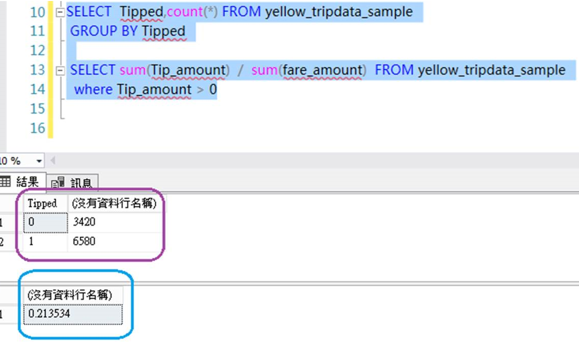
先直接看5種演算法練習最終比較準確度的結果,然後再開始實驗過程(載入資料、組成訓練組與測試組、訓練建模、預測、比較預測結果)。
看起來決策樹(0.99)和隨機森林(0.91)在這個資料情境下暫時領先
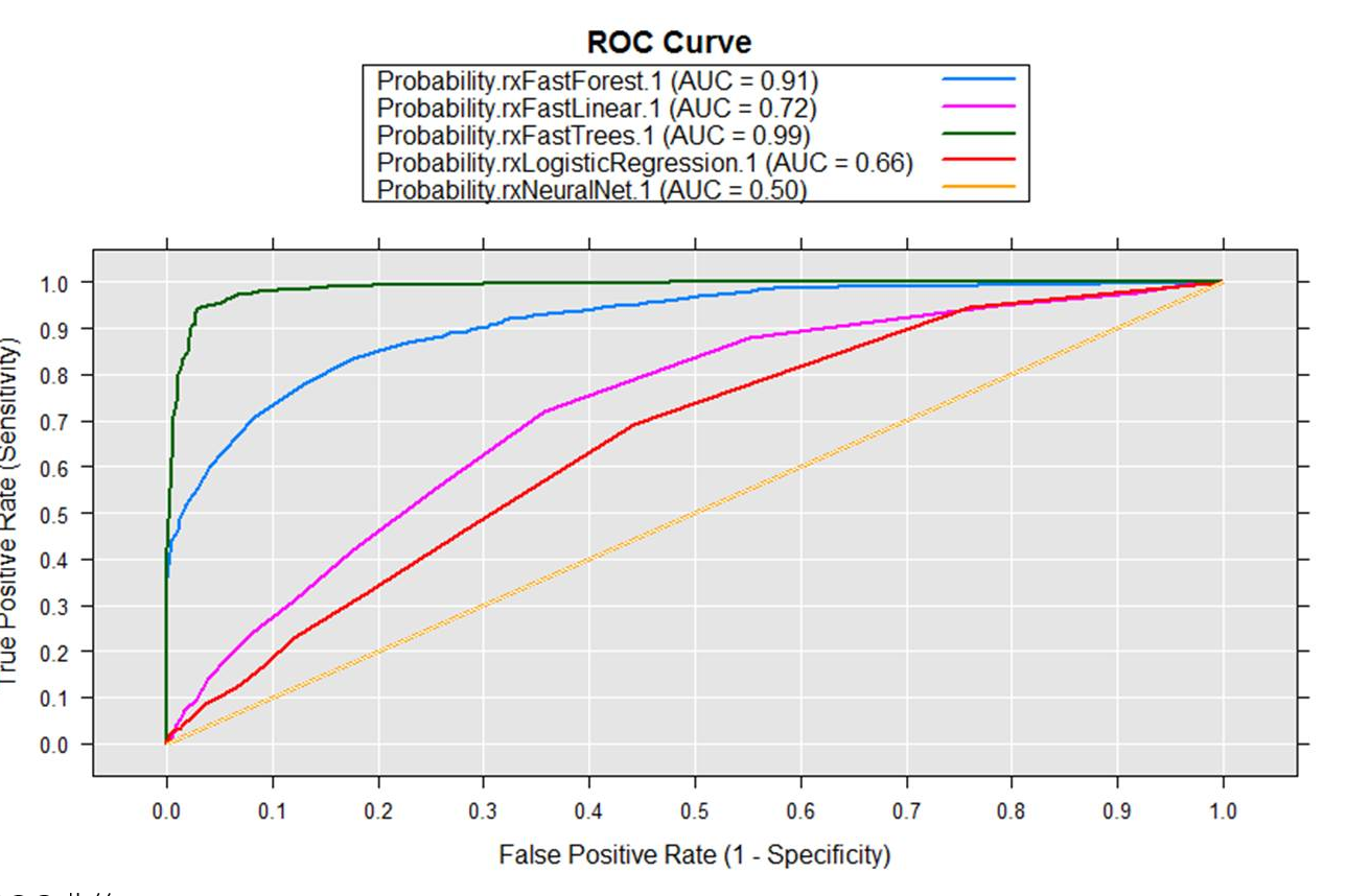
ROC曲線:
- X軸是FPR(False positive rate) FP / (FP + TN),也稱錯誤命中率、假警報的機率(false alarm rate),在所有沒有給小費的交易中,有多少被誤判有給。
- Y軸是TPR(True positive rate) TP/(TP+FN),也稱敏感度(sensitivity)或是命中率(Hit rate),有給小費的交易中,多少成功被預測有給小費。
資料集下載及匯入SQL Server
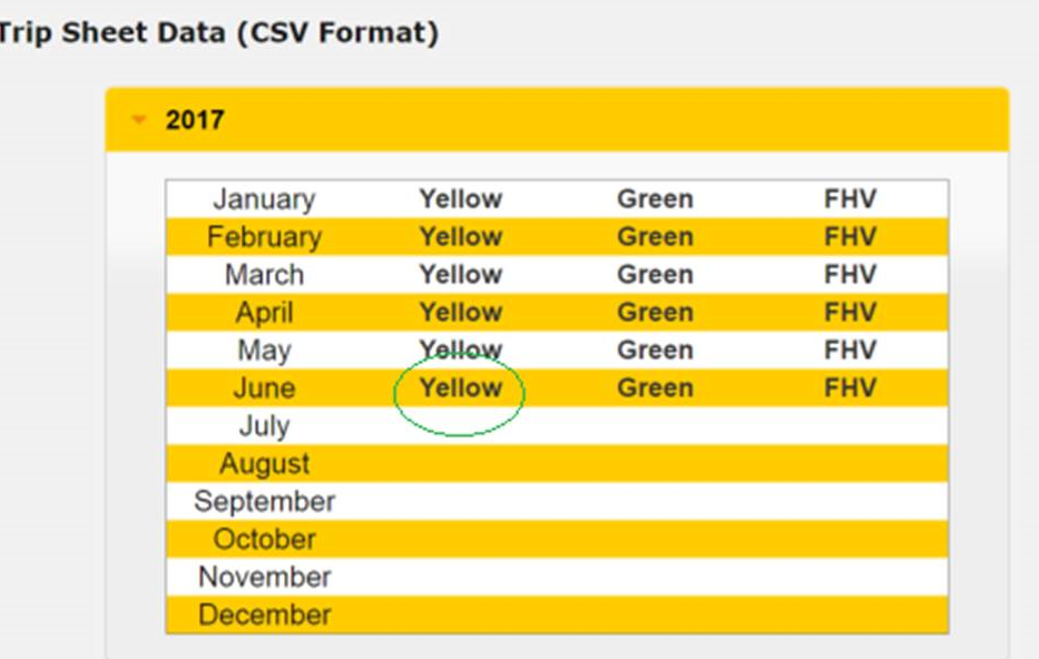
因為原本的資料集太大(3.8GB),我們改從紐約州政府網站下載(也可以從kaggle網站下載)。
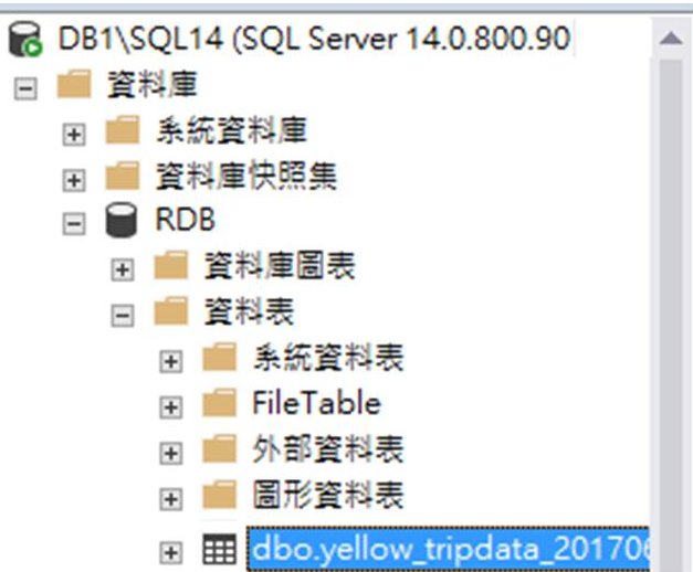
我們選擇下載2017年6月的黃牌計程車交易數據,交易資料大約900多萬筆,檔案大約812MB。
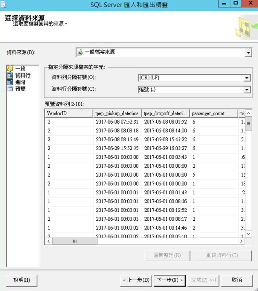
使用SQL管理工具匯入資料
預覽資料列
900多萬筆資料傳送且匯入完成,大約2分鐘
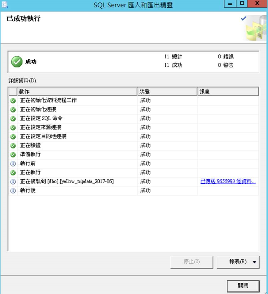
要測試的資料集載入SQL Server資料平台了!
資料集整理及抽樣
先簡單從yello-tripdata-2016-06 抽樣(sampling) 1萬筆資料,並且用T-SQL整理資料。
CREATE TABLE dbo.yellow_tripdata_sample
           (
           VendorID varchar(50) NULL,
           tpep_pickup_datetime varchar(50) NULL,
           tpep_dropoff_datetime varchar(50) NULL,
           passenger_count int NULL,
           trip_distance decimal(13, 2) NULL,
           RatecodeID varchar(50) NULL,
           store_and_fwd_flag varchar(50) NULL,
           PULocationID varchar(50) NULL,
           DOLocationID varchar(50) NULL,
           payment_type varchar(50) NULL,
           fare_amount decimal(13, 2) NULL,
           extra varchar(50) NULL,
           mta_tax decimal(13, 2) NULL,
           tip_amount decimal(13, 2) NULL,
           tolls_amount decimal(13, 2) NULL,
           improvement_surcharge varchar(50) NULL,
           total_amount decimal(13, 2) NULL,
           tipped int null,
           trip_time_in_secs int
           )  ON [PRIMARY]
GO


INSERT INTO dbo.yellow_tripdata_sample
SELECT top 10000
VendorID
,tpep_pickup_datetime
,tpep_dropoff_datetime
, CONVERT(int, passenger_count) as passenger_count
, CONVERT(decimal(13, 2), trip_distance) as trip_distance
, RatecodeID
, store_and_fwd_flag
, PULocationID
, DOLocationID
, payment_type
, CONVERT(decimal(13, 2), fare_amount) as fare_amount
, extra
, CONVERT(decimal(13, 2), mta_tax) as mta_tax
, CONVERT(decimal(13, 2), tip_amount) as tip_amount
, CONVERT(decimal(13, 2), tolls_amount) as tolls_amount
, improvement_surcharge
, CONVERT(decimal(13, 2), [total_amount ])  as total_amount
, case WHEN CONVERT(decimal(13, 2), tip_amount) > 0 THEN 1 ELSE 0 END AS tipped
, DATEDIFF(second,tpep_pickup_datetime,tpep_dropoff_datetime) AS trip_time_in_secs
FROM dbo.[yellow_tripdata_2017-06]
先用小資料把程式寫好,再一口氣來大資料。
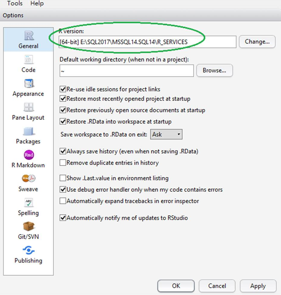
R Studio(確認 R Runtime)
從測試DB Server打開R Studio,確認R Version(Tools > Global option)
執行R Script
萬事俱備,來執行R語言了!
共有8個步驟,依序從載入Library(1)、載入資料集(2)、資料分組(3)、設定方程式(4)、訓練建模(5)、預測(6)、比較(7)、尋找最佳(8)。
Tiger team blog的R範例,我們只稍改了一下資料庫連線字串和資料表名稱
#####################################
#Step 1: Load the MicrosoftML package
#####################################
library(MicrosoftML)

#####################################
#Step 2: Import Data
#####################################
sqlConnString <- "Driver=SQL Server;Server=DB1\\SQL14;Database=RDB;Trusted_Connection=True"
dataSetSource <- RxSqlServerData(connectionString = sqlConnString, table = "yellow_tripdata_sample", rowsPerRead = 2000000)
dataset <- rxImport(dataSetSource)
rxGetVarInfo(dataset)

#####################################
#Step 3: Split Dataset into Train and Test
#####################################

# Set the random seed for reproducibility of randomness.
set.seed(2345, "L'Ecuyer-CMRG")
# Randomly split the data 75-25 between train and test sets.
dataProb <- c(Train = 0.75, Test = 0.25)
dataSplit <-
  rxSplit(dataset,
          splitByFactor = "splitVar",
          transforms = list(splitVar =
                              sample(dataFactor,
                                     size = .rxNumRows,
                                     replace = TRUE,
                                     prob = dataProb)),
          transformObjects =
            list(dataProb = dataProb,
                 dataFactor = factor(names(dataProb),
                                     levels = names(dataProb))),
          outFilesBase = tempfile())

# Name the train and test datasets.
dataTrain <- dataSplit[[1]]
dataTest <- dataSplit[[2]]
rxSummary(~ tipped, dataTrain)$sDataFrame
rxSummary(~ tipped, dataTest)$sDataFrame

#####################################
#Step 4: Define Model
#####################################
model <- formula(paste("tipped ~ passenger_count + trip_time_in_secs + trip_distance + total_amount"))

#####################################
#Step 5: Fit Model
#####################################
rxLogisticRegressionFit <- rxLogisticRegression(model, data = dataTrain)
rxFastLinearFit <- rxFastLinear(model, data = dataTrain)
rxFastTreesFit <- rxFastTrees(model, data = dataTrain)
rxFastForestFit <- rxFastForest(model, data = dataTrain)
rxNeuralNetFit <- rxNeuralNet(model, data = dataTrain)

#####################################
#Step 6: Predict
#####################################
fitScores <- rxPredict(rxLogisticRegressionFit, dataTest, suffix = ".rxLogisticRegression",
                       extraVarsToWrite = names(dataTest),
                       outData = tempfile(fileext = ".xdf"))
fitScores <- rxPredict(rxFastLinearFit, fitScores, suffix = ".rxFastLinear",
                       extraVarsToWrite = names(fitScores),
                       outData = tempfile(fileext = ".xdf"))
fitScores <- rxPredict(rxFastTreesFit, fitScores, suffix = ".rxFastTrees",
                       extraVarsToWrite = names(fitScores),
                       outData = tempfile(fileext = ".xdf"))
fitScores <- rxPredict(rxFastForestFit, fitScores, suffix = ".rxFastForest",
                       extraVarsToWrite = names(fitScores),
                       outData = tempfile(fileext = ".xdf"))
fitScores <- rxPredict(rxNeuralNetFit, fitScores, suffix = ".rxNeuralNet",
                       extraVarsToWrite = names(fitScores),
                       outData = tempfile(fileext = ".xdf"))

#####################################
#Step 7: Compare Models
#####################################
# Compute the fit models's ROC curves.
fitRoc <- rxRoc("tipped", grep("Probability.", names(fitScores), value = T), fitScores)
# Plot the ROC curves and report their AUCs.
plot(fitRoc)


#####################################
#Step 8: Find the best fit using AUC values
#####################################
# Create a named list of the fit models.
fitList <-
  list(rxLogisticRegression = rxLogisticRegressionFit,
       rxFastLinear = rxFastLinearFit,
       rxFastTrees = rxFastTreesFit,
       rxFastForest = rxFastForestFit,
       rxNeuralNet = rxNeuralNetFit)

# Compute the fit models's AUCs.
fitAuc <- rxAuc(fitRoc)
names(fitAuc) <- substring(names(fitAuc), nchar("Probability.") + 1)

# Find the name of the fit with the largest AUC.
bestFitName <- names(which.max(fitAuc))

# Select the fit model with the largest AUC.
bestFit <- fitList[[bestFitName]]

# Report the fit AUCs.
cat("Fit model AUCs:\n")
print(fitAuc, digits = 2)

# Report the best fit.
cat(paste0("Best fit model with ", bestFitName,
           ", AUC = ", signif(fitAuc[[bestFitName]], digits = 2),
           ".\n"))
最後利用內建的RxAUC函數輕輕鬆鬆劃出ROC曲線
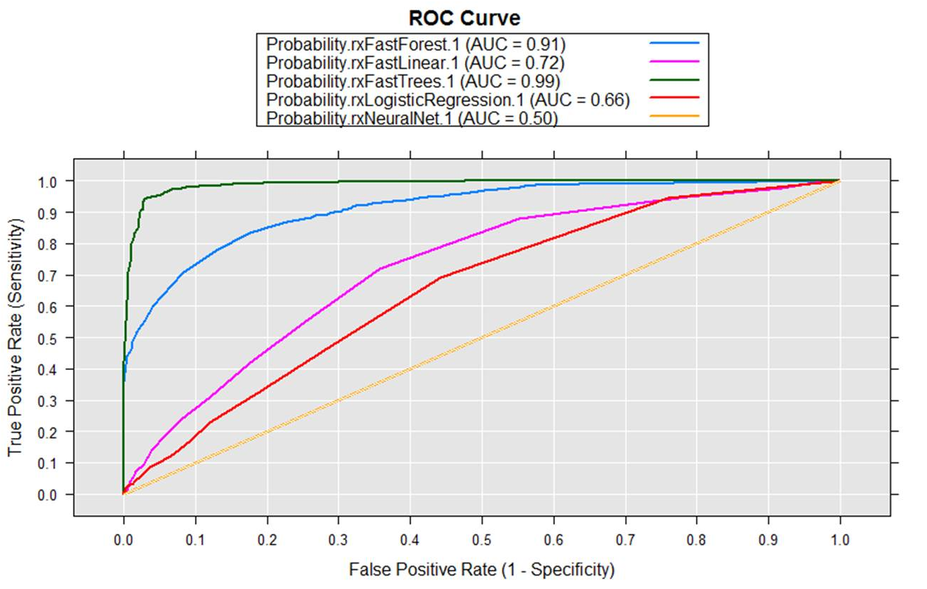
ROC曲線下方的面積稱為AUC(Area under the Curve of ROC),中間的直線就是AUC=0.5,這次剛好是類神經網路;模型的AUC值越高,正確率越高。在這個資料情境及抽樣下,決策樹與隨機森林準確度很高,反倒是類神經網路、線性與迴歸表現較不理想。
這邊也從郭耀仁老師iThome鐵人賽文章找到一個AUC值對照預測效果的形容詞
| AUC區間 | 1-0.9 | 0.9-0.8 | 0.8-0.7 | 0.7-0.6 | 0.6-0.5 |
| 效果 | 傑出 | 優秀 | 普通 | 不好 | 差 |
小結
Stored Procedure(external script):
也可以用Stored Procedure(external script)執行,但因為語法比較長,不容易Debug,建議包成package或先用R Studio測試過再執行。
其他比較演算法準確度的方式:
在這些分類性的問題中,除了視覺化AUC曲線比較各種演算法外,整體準確率(Accuracy)或是組合混淆矩陣(confusion matrix)中的其他資訊的精確率(precision)、命中率(Hit rate)以及F1 Score(前兩者的數學調和平均)也都是常用的比較方式。
參考
redicting NYC Taxi Tips using MicrosoftML
rxRoc: Receiver Operating Characteristic (ROC) computations and plot
rxLogisticRegression: Logistic Regression
rxFastLinear: Fast Linear Model -- Stochastic Dual Coordinate Ascent